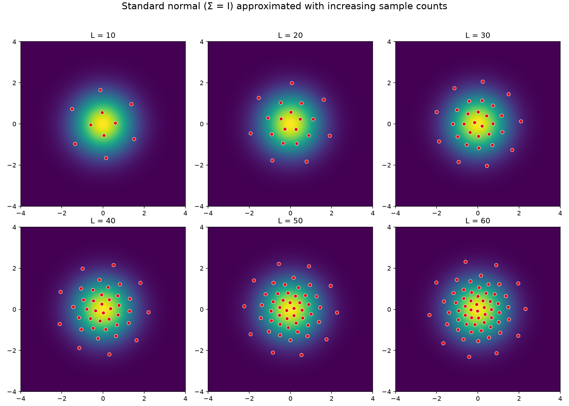
These plots show deterministic LCD / Dirac-mixture approximations of 2-D Gaussian densities. In each panel the shaded field is the target Gaussian density and the red points are the optimized deterministic sample (Dirac) locations produced by the gm_to_dirac_short sampler.
Within the framework of the Gaussian-to-Dirac approximation, the covariance matrix \( \Sigma \in R^{N×N} \) is first spectrally decomposed:
where \( Q \) is orthogonal and \( \Lambda = \text{diag}(\lambda_1, \ldots, \lambda_N) \) contains the positive eigenvalues. This transformation diagonalizes the covariance and eliminates inter-dimensional correlation, allowing optimization to be performed in an uncorrelated, axis-aligned coordinate system. The optimization of the Dirac support points is thus carried out in the diagonalized coordinate system with covariance \( \Lambda \). Upon completion of the optimization, the support points \( z_i \) determined in the transformed space are mapped back to the original coordinate system via \( x_i = Q z_i \).
Correlated covariances
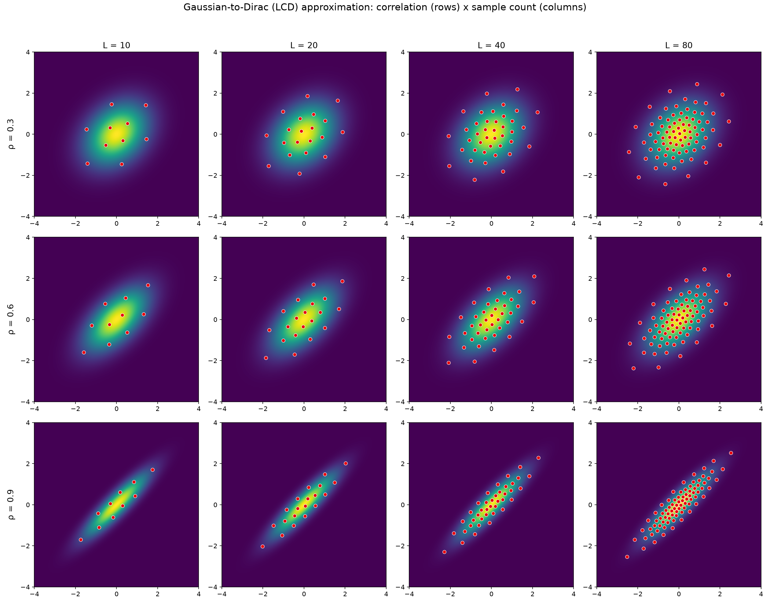
The grid sweeps both correlation and sample count for the unit-variance covariance \( \Sigma = \begin{bmatrix} 1 & \rho \\ \rho & 1 \end{bmatrix} \).
Standard normal scaling